Python Big O Notation

The same program runs fast on a new computer and slow on an old one. So seconds are a bad way to compare two algorithms — the number depends on the machine, not only on the code.

Instead we count steps: how many simple operations the algorithm does. A step is one small action, like reading a value, comparing two numbers, or adding them.

Big O notation describes how the number of steps grows when the input grows. It does not say "this takes 3 seconds". It says "if the input doubles, the work doubles" — that is O(n) — or "if the input doubles, the work stays the same" — that is O(1).

Big O looks at the worst case: the most steps the algorithm can ever need for an input of size n.

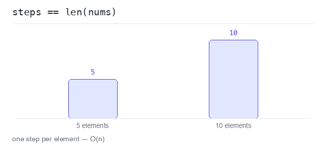
A loop that visits every element of a list does one pass per element. For 5 elements that is 5 steps, for 10 elements 10 steps. The step count is the same as len(nums).

We do not care about the exact number. We care about the shape of the growth: twice the input, twice the steps. That shape is called linear, written O(n).

The function increases a steps counter inside the loop. A list of 5 elements takes 5 steps, a list of 10 elements takes 10 steps — the count follows the input size.

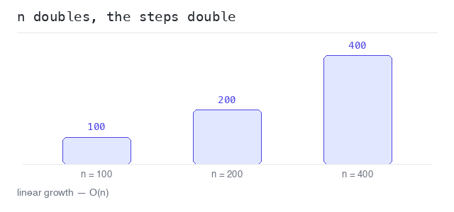
The program runs the same counting loop for n = 100, 200 and 400. Every time n doubles, the step count doubles too. That is the fingerprint of O(n).

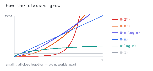
Most algorithms fall into a few common growth classes, from fastest to slowest:

O(1) constant — the work never grows.
O(log n) logarithmic — doubling the input adds only one step.
O(n) linear — the work grows with the input.
O(n log n) — a good sorting algorithm.
O(n²) quadratic — a loop inside a loop.
O(2ⁿ) exponential — the work doubles with every extra element.

For small inputs the difference is tiny. For big inputs it decides whether the program answers at once or never finishes.

The table shows the step counts for growing n. At n = 16, log n is only 4 while 2ⁿ is already 65536. The bigger n gets, the more the classes drift apart.

Big O keeps only the shape of the growth and throws the details away. O(2n), O(n + 5) and O(n) are all the same class: linear.

Why? Because for big inputs the constant factor stops mattering. An algorithm that does 2 passes over a million elements is still in a different world than one that compares every element with every other element.

The exact rules for simplifying — drop the constants, drop the smaller terms — have their own page later in this group.

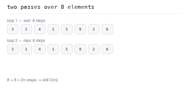
The program does two separate passes over the list: one for the sum, one for the biggest value. That is 2n steps — 16 for 8 elements. Big O drops the constant 2, so this is still O(n).